Mathematics · 2023

Exponentiation
by Matrices

How eigendecomposition turns a matrix differential equation into a closed-form solution, and what phase portraits reveal about long-run behavior. Advanced Topics Math, 2023.

Given a matrix $A$ and an initial state $x_{0} \in R^{n}$ , the differential equation $\overset{x}{˙} = A x$ has the exact solution $x (t) = e^{A t} x_{0}$ . The catch: computing the matrix exponential directly is expensive. Eigendecomposition provides a shortcut that reduces the problem to scalar exponentials, one per eigenvalue of $A$ .

This project builds the intuition from first principles, implements interactive phase-plane visualizations in Python, and explores how the sign and magnitude of eigenvalues dictate qualitatively different long-run behaviors.

Context

Advanced Topics Mathematics, senior year

Tools

PythonNumPyMatplotlibipywidgets

Topics

Eigendecomposition · matrix exponential · phase planes · linear ODEs · Euler's method

The Problem

A linear autonomous system is a differential equation of the form:

System of ODEs

\overset{x}{˙} = A x, x (0) = x_{0}

where $A \in R^{n \times n}$ is a constant matrix and $x (t) \in R^{n}$ is the state we want to find. In 2D this describes trajectories in the plane. Each point $(x_{1}, x_{2})$ has a velocity $\overset{x}{˙} = A [x_{1} x_{2}]$ attached to it, forming a vector field.

The exact solution is the matrix exponential:

Exact solution

x (t) = e^{A t} x_{0}

This generalizes the scalar case: when $A = a \in R$ , the solution to $\overset{x}{˙} = a x$ is $x (t) = e^{a t} x_{0}$ .

The matrix exponential is defined by a power series:

Definition

e^{A t} = k = 0 \sum \infty \frac{( A t ) ^{k}}{k !} = I + A t + \frac{A ^{2} t ^{2}}{2 !} + \dots

This converges for any square matrix $A$ , but computing many matrix powers is $O (n^{3})$ per term — expensive. Eigendecomposition replaces those matrix multiplications with cheap scalar ones.

Key property

If $A = V Λ V^{- 1}$ , then $e^{A t} = V e^{Λ t} V^{- 1}$ . The matrix exponential inherits the eigenstructure of $A$ .

Eigendecomposition

A nonzero vector $v$ is an eigenvector of $A$ if applying $A$ only scales it, never rotates it:

Eigenvalue equation

A v = λ v

Collecting eigenvectors as columns of $V = [v_{1} ∣ \dots ∣ v_{n}]$ and eigenvalues on the diagonal of $Λ = diag (λ_{1}, \dots, λ_{n})$ :

Matrix form

A V = V Λ ⟹ A = V Λ V^{- 1}

This holds whenever $A$ has $n$ linearly independent eigenvectors (the diagonalizable case, which covers most matrices in practice).

Substituting $A = V Λ V^{- 1}$ into the power series, every $A^{k} = V Λ^{k} V^{- 1}$ , so:

Key simplification

e^{A t} = V (k = 0 \sum \infty \frac{( Λ t ) ^{k}}{k !}) V^{- 1} = V e^{Λ t} V^{- 1}

Because $Λ$ is diagonal, its exponential is just:

Diagonal matrix exponential

e^{Λ t} = e^{λ_{1} t} ⋱ e^{λ_{n} t}

The full closed-form solution is:

Closed-form solution

x (t) = V diag (e^{λ_{1} t}, \dots, e^{λ_{n} t}) V^{- 1} x_{0}

Three-Step Computation

Solution steps

Computing

x (t) = e^{A t} x_{0}

in three steps: (1) project

x_{0}

into the eigenvector basis with

V^{- 1}

; (2) apply scalar growth/decay

e^{λ_{i} t}

along each eigendirection; (3) project back with

V

Scalar exponentials

The diagonal entries of

e^{Λ t}

. Negative eigenvalues produce exponential decay (stable modes); positive ones grow without bound (unstable modes). The rate is

∣ λ ∣

, the time constant

1/∣ λ ∣

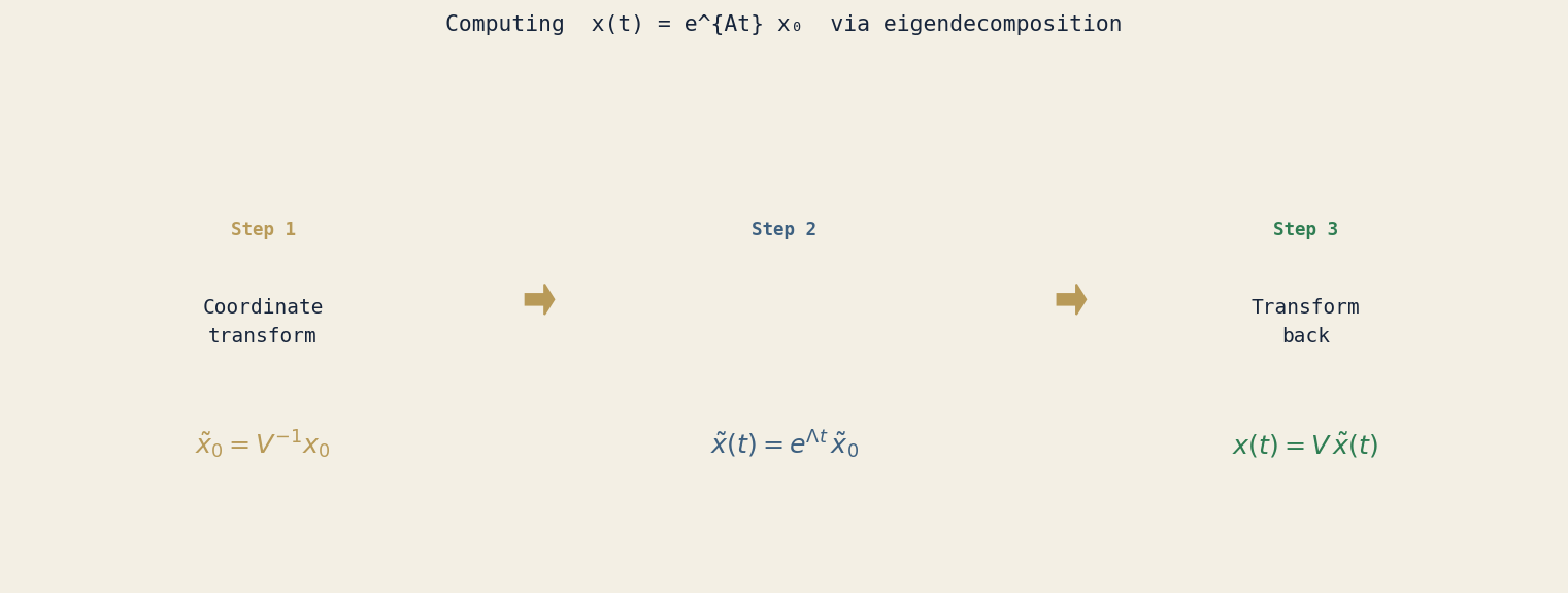
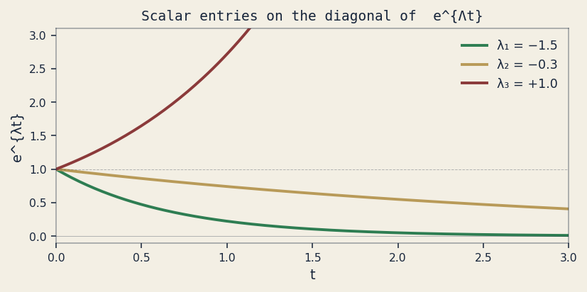
In the eigenvector basis $\tilde{x} = V^{- 1} x$ , the system decouples completely:

Decoupled in eigenbasis

\dot{\tilde{x}} = Λ \tilde{x} ⟹ \tilde{x}_{i} (t) = e^{λ_{i} t} \tilde{x}_{i} (0)

Each coordinate $\tilde{x}_{i}$ evolves independently as a scalar exponential. Coupling only reappears when projecting back into the original basis with $V$ .

Equivalently, the solution is a superposition of modes:

Modal decomposition

x (t) = i = 1 \sum n c_{i} e^{λ_{i} t} v_{i}, c = V^{- 1} x_{0}

Each mode $e^{λ_{i} t} v_{i}$ decays or grows along its eigenvector direction. Long-run behavior is dominated by the mode with the largest real part of $λ_{i}$ .

Phase Portraits

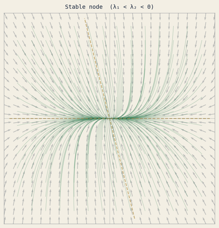
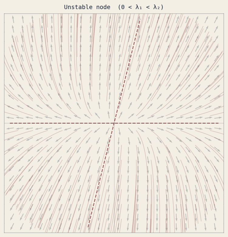
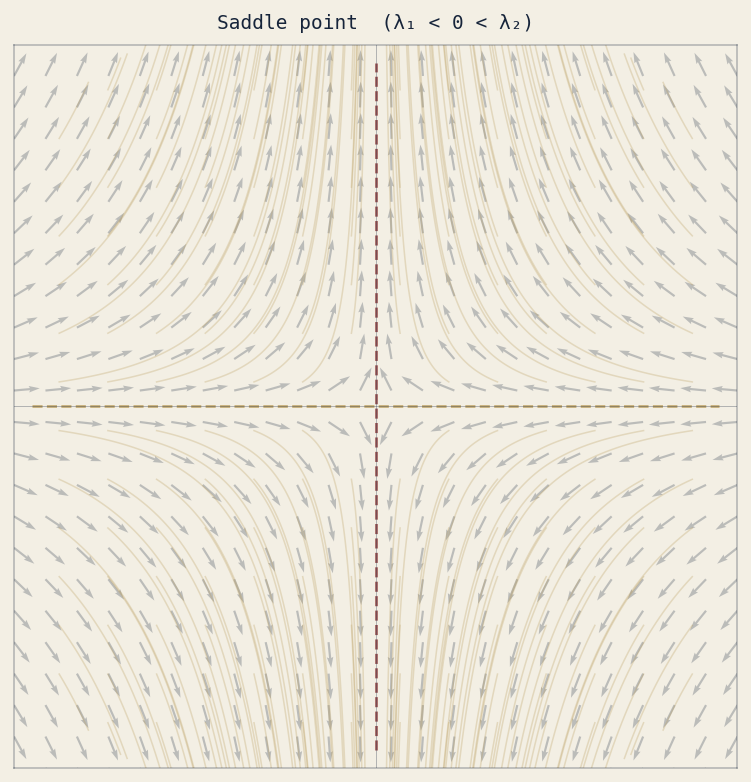
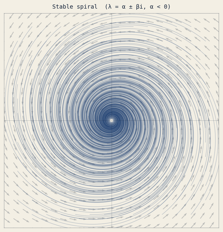
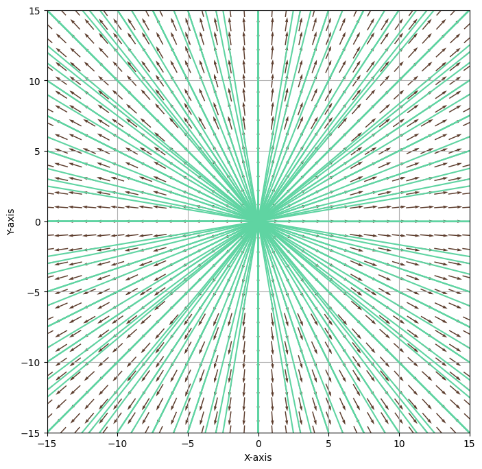
A phase portrait overlays the vector field $\overset{x}{˙} = A x$ with solution curves for many initial conditions simultaneously. The qualitative shape — whether trajectories converge, diverge, spiral, or oscillate — is entirely determined by the eigenvalues of $A$ . Dashed lines mark eigenvector directions.

Stable node

Stable node: both eigenvalues real and negative,

λ_{1} < λ_{2} < 0

. All trajectories converge to the origin. Near the origin, curves align with the slower eigenvector (smaller

∣ λ ∣

Unstable node

Unstable node: both eigenvalues real and positive,

0 < λ_{1} < λ_{2}

. Trajectories diverge from the origin. Equivalent to replacing

A

with

- A

in the stable case.

Saddle point

Saddle point: eigenvalues of opposite sign,

λ_{1} < 0 < λ_{2}

. Trajectories are attracted along the stable manifold (gold dashes) and repelled along the unstable manifold (red dashes). Almost all initial conditions eventually escape to infinity.

Stable spiral

Stable spiral: complex eigenvalues

λ = α \pm β i

with

α < 0

. Trajectories rotate with angular frequency

β

while decaying at rate

∣ α ∣

. Pure imaginary (

α = 0

) gives closed orbits — a center.

Project: convergent field

Phase portrait from the project. The matrix

A

was constructed interactively by entering two eigenvectors and eigenvalues; the code reconstructed

A = V Λ V^{- 1}

and plotted the resulting vector field and integral curves in real time.

Project: Euler's method path

The orange path traces a single solution using Euler's method with step size

h = 0.01

. Each step computes

x_{k + 1} = x_{k} + h A x_{k}

, following the vector field numerically. At small

h

this closely matches the analytic solution

x (t) = e^{A t} x_{0}

Euler's Method

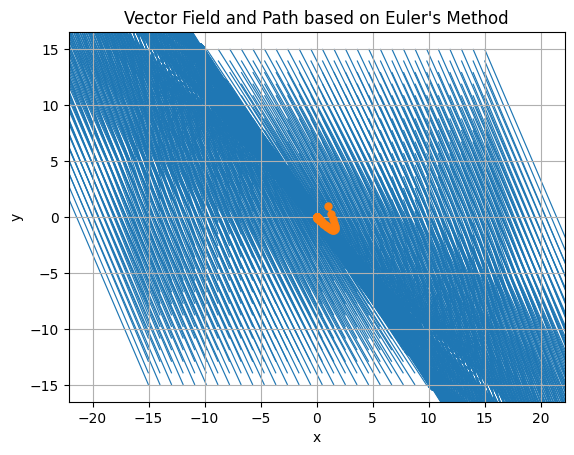
Euler's method approximates the solution by taking small linear steps along the vector field:

Euler update rule

x_{k + 1} = x_{k} + h A x_{k} = (I + h A) x_{k}

After $N$ steps of size $h = t / N$ :

N steps

x (t) \approx (I + \frac{t}{N} A)^{N} x_{0} N \to \infty e^{A t} x_{0}

This limit is exactly the compound-interest definition of the exponential, now applied to matrices. It connects numerical integration directly to the analytic formula.

Euler integration (forward + backward)

def generate_path(x0, A, steps=1000):
    fwd = [x0]
    for _ in range(steps):           # forward in time
        fwd.append(fwd[-1] + A @ fwd[-1] / steps)

    bwd = [x0]
    for _ in range(steps):           # backward in time
        bwd.append(bwd[-1] - A @ bwd[-1] / steps)

    return np.concatenate([bwd[::-1], fwd[1:]])

Build the vector field

X, Y = np.meshgrid(np.arange(-15, 16), np.arange(-15, 16))
U = A[0,0]*X + A[0,1]*Y   # ẋ₁ = a₁₁x₁ + a₁₂x₂
V = A[1,0]*X + A[1,1]*Y   # ẋ₂ = a₂₁x₁ + a₂₂x₂
mag = np.hypot(U, V)
ax.quiver(X, Y, U/mag, V/mag, pivot='mid')

Reconstructing A from Eigenpairs

The interactive part of the project lets a user specify eigenvectors and eigenvalues directly. Given $v_{1}, v_{2}$ and $λ_{1}, λ_{2}$ :

Reconstruction

A = V Λ V^{- 1} = [v_{1} v_{2}] [λ_{1} 0 0 λ_{2}] [v_{1} v_{2}]^{- 1}

The resulting $A$ is guaranteed to have exactly those eigenpairs. Flipping eigenvalue signs immediately transforms a stable phase portrait into an unstable one — making the connection between eigenvalues and long-run behavior viscerally clear.

Reconstruct A from eigenpairs

def make_A(eigenvectors, eigenvalues):
    V      = np.column_stack(eigenvectors)
    Lambda = np.diag(eigenvalues)
    return V @ Lambda @ np.linalg.inv(V)   # A = V Λ V⁻¹

# Stable node: both eigenvalues negative
A = make_A([[1, 0], [0, 1]], [-1, -3])
# → [[-1,  0],
#    [ 0, -3]]

# Saddle: mixed signs
A = make_A([[1, 0], [0, 1]], [-1, 2])
# → [[-1,  0],
#    [ 0,  2]]

Key Takeaway

The solution to $\overset{x}{˙} = A x$ is entirely determined by the eigenstructure of $A$ . Each eigenvalue $λ_{i}$ contributes a mode $c_{i} e^{λ_{i} t} v_{i}$ to the solution. Negative real parts produce decay; positive real parts produce growth; imaginary parts produce oscillation. The phase portrait makes all three readable at a glance.

x (t) = i \sum c_{i} e^{λ_{i} t} v_{i}, c = V^{- 1} x_{0}

Exponentiationby Matrices

Exponentiation
by Matrices